Radial Power Spectra: Quantifying the Pi Matrix Across Scales

Allen, James Johan Sebastian

Radial Power Spectra: Quantifying the Pi Matrix Across Scales

By James Johan Sebastian Allen — PatternFieldTheory.com • Last updated: 2025-10-05

Images from field ion microscopy (FIM), transmission electron microscopy (TEM), scanning tunneling / atomic force microscopy (STM/AFM) — and even full-sky maps — contain hidden structure in their frequency domain. By computing the radial power spectrum we can operationally quantify coherence, scale-coupling, and fractal-like behavior attributed in PFT™ to the Pi Matrix, from sub-nanometer lattices to sky-scale maps.

1) Pipeline — from pixels to $P(k)$

Preprocess: grayscale/intensity image $I(x,y)$; remove large-scale gradients (high-pass or polynomial detrend); apply apodization (Hann/Hamming) to reduce edge leakage.
Fourier transform: compute $F(k_x,k_y)=\mathcal{F}\{I(x,y)\}$ and the 2D power $P(k_x,k_y)=|F(k_x,k_y)|^2$.
Radial average: bin by $k=\sqrt{k_x^2+k_y^2}$ to obtain the 1D spectrum $P(k)=\langle |F|^2\rangle_\theta$.
Fit slope: on log–log axes, fit a line to $\log P$ vs. $\log k$ over a chosen inertial band to estimate the exponent $\beta$.

Definitions
Fourier power: $ P(k_x,k_y)=|F(k_x,k_y)|^2 $.
Radial spectrum: $ P(k)=\langle P(k_x,k_y)\rangle_{\theta} $ with $ k=\sqrt{k_x^2+k_y^2} $.

2) Interpreting slopes

In many textures, $P(k)\propto k^{-\beta}$. Within PFT’s framing, steeper slopes (larger $\beta$) indicate stronger long-range coherence (energy concentrated at low spatial frequencies), while shallower slopes suggest more local structure.

About “fractal dimension” mappings
Different communities use different conventions. For self-affine 2D fields and surfaces, $\beta$ relates to a Hurst-like exponent $H$ via forms such as $ \beta \approx 2H+E $ (with $E$ the embedding dimension used for the PSD), while “effective fractal dimension” $D$ is defined contextually (e.g., for surfaces, $D\approx E+1-H$). In this article we use $\beta$ primarily as a coherence scale index; any quoted $D$ should state the convention and embedding explicitly.

3) Case sketches

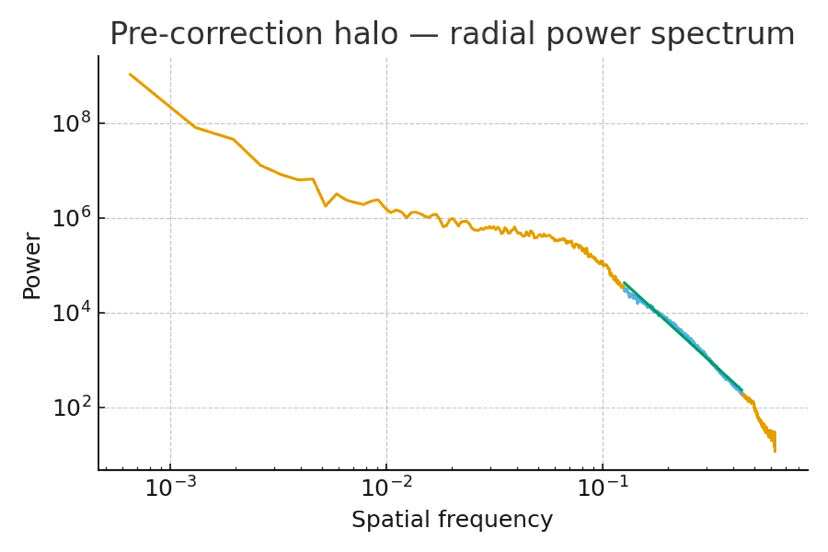
Pre-correction halo

Early TEM/FIM images sometimes show halos/blur. PFT interprets these as a living cascade: resonance updating faster than optics can freeze. Radial spectra typically show enhanced low-$k$ power and a persistent slope.

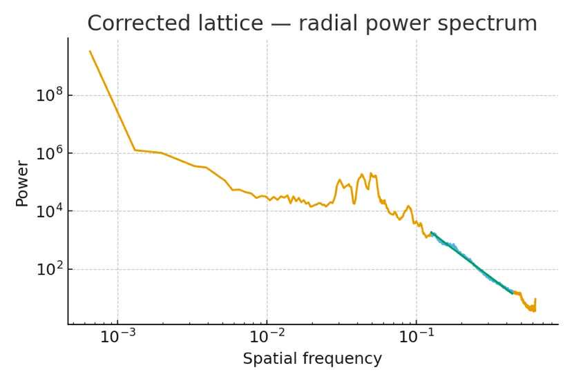
Corrected lattice

With aberration correction, the motion freezes into a crisp lattice. High-$k$ power is suppressed; the radial slope flattens at the upper band — a Zeno frame snapshot in PFT language.

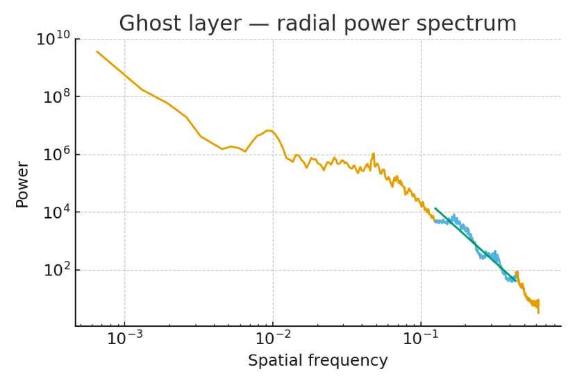
Ghost / logical layer

Subtle understructures (post-processing residuals or phase-like “ghosts”) can retain scale-invariant slopes, interpreted as a guiding logical layer in PFT’s ontology.

Radial spectrum of ghost layer — Ghost-layer spectrum — scale-invariant residuals beneath atomic order.

Blurry pre-correction

Before correction, blurred cascades often show strong power across decades in $k$, consistent with active resonance/transport.

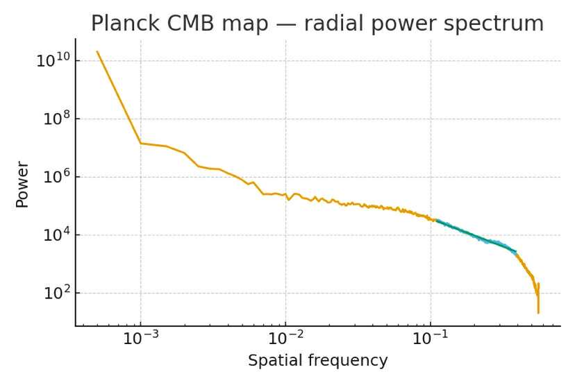
4) From atoms to sky maps

The same pipeline applies to large-scale maps (e.g., full-sky intensity/polarization). While the geometry differs (spherical harmonics $C_\ell$ versus planar $P(k)$), both quantify how power distributes with scale. In PFT, similar slope behaviors across domains are taken as suggestive of a common substrate (Pi Matrix) — a hypothesis to be tested with consistent masks, beams, and noise models.

5) Reproducibility checklist

State the image source and pixel scale (e.g., nm/pixel, arcmin/pixel).
Document detrending, windowing, and any deconvolution/PSF handling.
Publish binning scheme for $k$ and the exact fit band used for $\beta$.
Provide confidence intervals for $\beta$ (e.g., robust linear fit in log–log, bootstrap over tiles).
For sky maps: report masks, beams, and convert $C_\ell \leftrightarrow P(k)$ only with explicit approximations.

6) Compact formulas (operational)

$ F(k_x,k_y)=\mathcal{F}\{I(x,y)\}, \quad P(k_x,k_y)=|F(k_x,k_y)|^2 $
$ P(k)=\langle P(k_x,k_y)\rangle_{\theta}, \quad P(k)\propto k^{-\beta} $

Optional self-affinity sketch (declare convention): $ \beta \approx 2H + E $, with $E$ the embedding used for the PSD. Use $\beta$ as your primary reported metric unless a specific fractal-dimension convention is warranted and clearly stated.

Conclusion

Radial power spectra bridge images and mathematics. Their slopes and scale-dependence provide a compact fingerprint of coherence. In the PFT view, recurring slope behavior across domains is consistent with a universal conversion substrate (Pi Matrix), while instrument specifics (PSF, masks, windows) explain deviations. The method is simple, portable, and falsifiable.

Pattern Field Theory